# A tibble: 6 × 32
   time driver driver_number lap_time lap_number stint pit_out_time pit_in_time
  <dbl> <chr>  <chr>            <dbl>      <dbl> <dbl>        <dbl>       <dbl>
1 3438. VER    1                 94.3          1     1          NaN         NaN
2 3531. VER    1                 93.1          2     1          NaN         NaN
3 3624. VER    1                 93.1          3     1          NaN         NaN
4 3717. VER    1                 93.5          4     1          NaN         NaN
5 3810. VER    1                 92.8          5     1          NaN         NaN
6 3903. VER    1                 92.9          6     1          NaN         NaN
# ℹ 24 more variables: sector1time <dbl>, sector2time <dbl>, sector3time <dbl>,
#   sector1session_time <dbl>, sector2session_time <dbl>,
#   sector3session_time <dbl>, speed_i1 <dbl>, speed_i2 <dbl>, speed_fl <dbl>,
#   speed_st <dbl>, is_personal_best <list>, compound <chr>, tyre_life <dbl>,
#   fresh_tyre <lgl>, team <chr>, lap_start_time <dbl>, lap_start_date <dttm>,
#   track_status <chr>, position <dbl>, deleted <lgl>, deleted_reason <chr>,
# fast_f1generated <lgl>, is_accurate <lgl>, session_type <chr>STAT-244-SC
Final Project Report
- May 8, 2025
- Eonbi Choi, Yerim Oh
F1 Miami Grand Prix 2024 Pit Stop Analysis
Abstract
In sports, data is collected to record athletes’ performances, which helps in making decisions to improve outcomes. In Formula 1 and other motorsports, tire management plays an important role in race strategy. Tires directly impact car performance as they are in contact with the track and transfers all the car’s power and movements to the track surface. Tire degradation influences major decisions such as pit stop timing during a race, where minor misjudgments can result in serious consequences in a fast-paced sports like Formula 1. Our study evaluates the relationship between pit stop laps and tire and lap information though employing linear regression models, cross validation, k-fold cross validation, and logistic regression. The objective is to improve pit stop timing prediction to facilitate effective strategic planning for optimizing pit stop timing, ultimately giving drivers a decisive advantage in race management.
Datasets
The data used in this study were obtained from the f1dataR R package that accesses Formula 1 data via the FastF1 Python library. The dataset includes lap-by-lap session data from the 2024 Miami Grand Prix and comprise 1,111 laps and 32 variables. These variables include driver details, lap times, pit in/out times, tire information, and track status. More detailed information about this package can be found in its API documentation.
- Last accessed date/time: April 28, 2025 16:51 PM
Variables
quantitative variable:
lap_time: recorded time to complete a lap (seconds)lap_number: lap number from which the telemetry data was recorded (number of laps)tyre_life: number of laps completed on a set of tires (number of laps)
categorical variable:
compound: type of tire used (SOFT, MEDIUM, HARD)pit_in: whether a driver made a pit stop during a lap (binary: 0 = no pit stop, 1 = pit stop occured)
Clean/Rearrange Data
Rearrange data to consist only the variables we are interested in
Check missing values
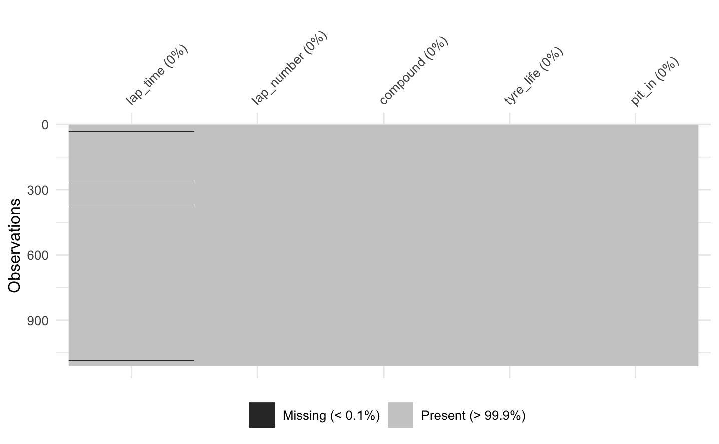
Data for lap_time are missing 5 values which are less than 0.1% of the entire observation
Finalize data we are going to use
# A tibble: 6 × 5
  lap_time lap_number compound tyre_life pit_in
     <dbl>      <dbl> <fct>        <dbl>  <dbl>
1     94.3          1 MEDIUM           1      0
2     93.1          2 MEDIUM           2      0
3     93.1          3 MEDIUM           3      0
4     93.5          4 MEDIUM           4      0
5     92.8          5 MEDIUM           5      0
6     92.9          6 MEDIUM           6      0
Why certain data points are missing
Out of 5 missing lap time records four records have a track status code of 41. However, no description of this code value is provided in the API. Thus, we assume that either the track was not fully cleared or conditions were not suitable for racing. The other missing record was due to a driver failing to complete a lap due to collision.
Data Visualization
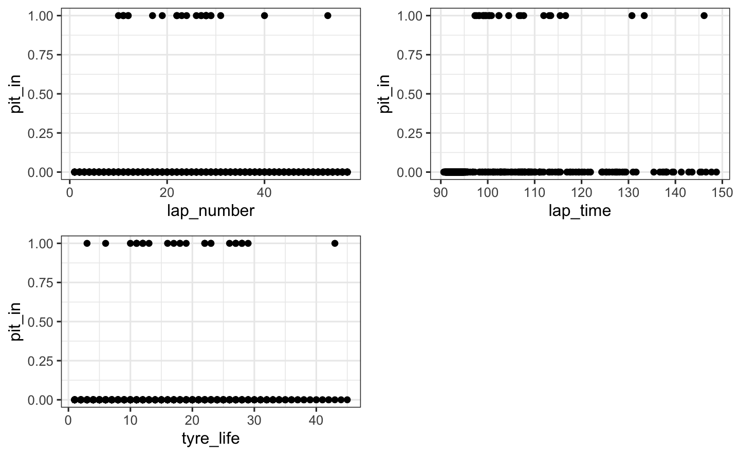
Our response variable:pit_in
Number of pit stops for each lap 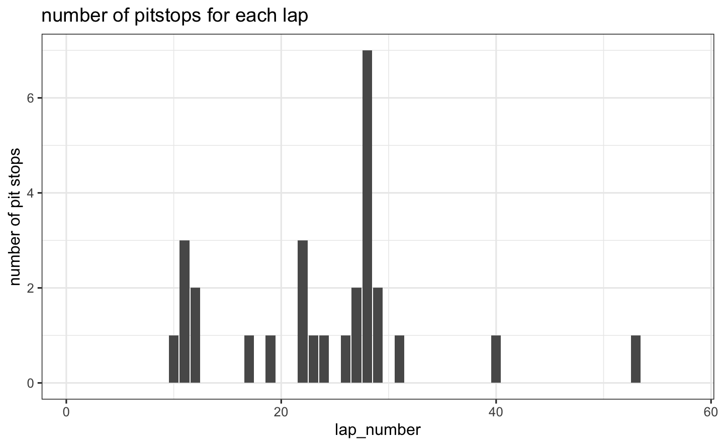 - This plot shows the frequency of pit stops across laps during the 2024 Miami Grand Prix. It helps visualize when teams tend to stop during the race. Many teams pitted to change tires during the first half of the race and the most common pit stop occurring around lap 28. This race was unique in that some drivers performed a one-stop strategy, while others went for a two-stop approach. These decisions were influenced by various factors such as track position, gaps to nearby drivers, tire condition, and more. Pit stops in the later stages of the race likely reflect either a two-stop strategy or an attempt to set the fastest lap and earn an extra point.
Density plot for lap time of each team 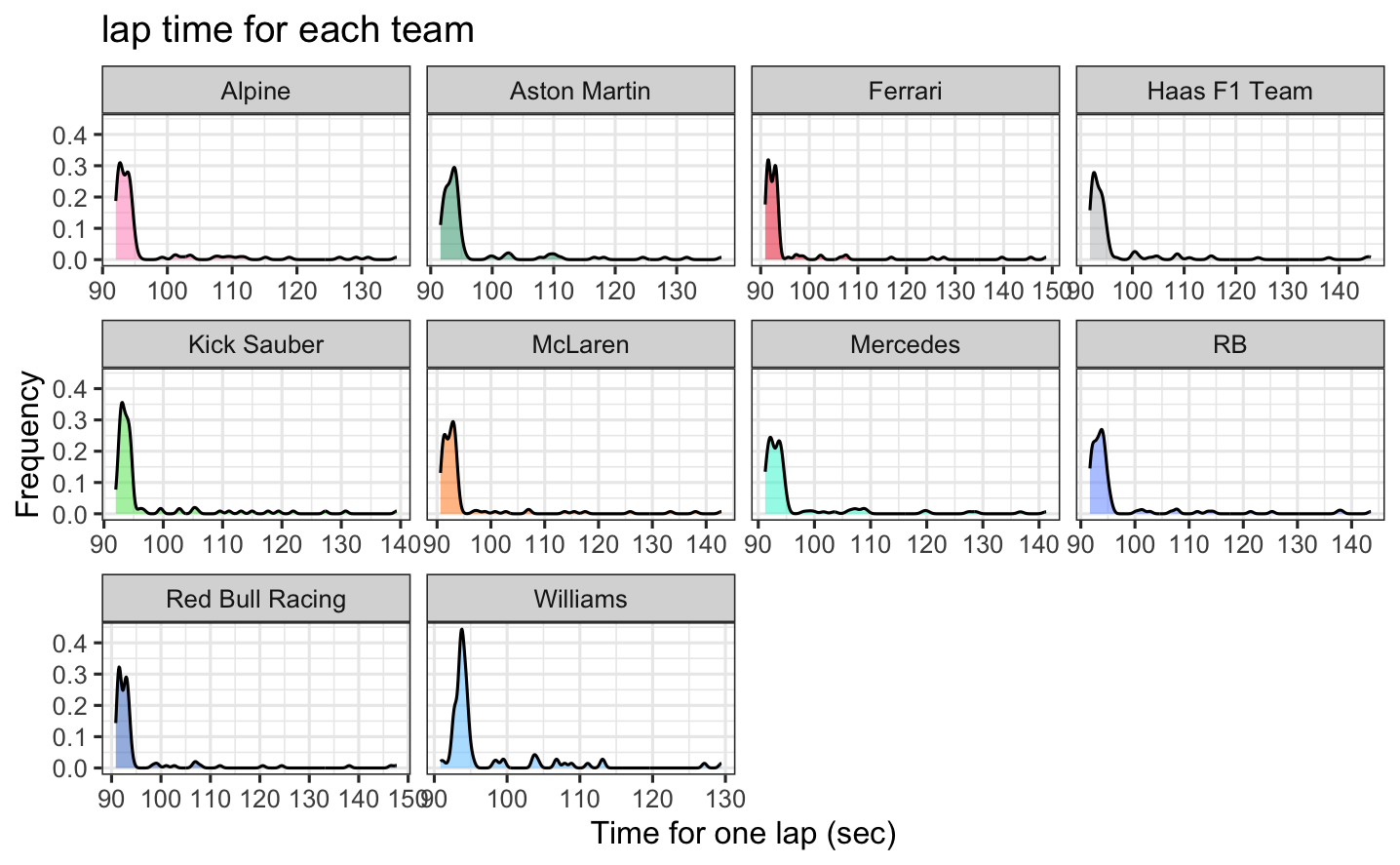 - This plot shows the distribution of lap times for each team during the race. We can compare the performance and variability in lap times across different teams. For most teams, the lap times are generally under 100 seconds, with some laps approaching 110 seconds. These patterns are largely consistent across teams, though some, such as Mercedes and Williams, show a few outliers on the higher end, which indicates occasional slower laps. - A smaller lap time in Formula 1 means that the driver completed a lap more quickly. In racing, lower lap times are better because they indicate higher performance.
Box plot of tire life for each compound 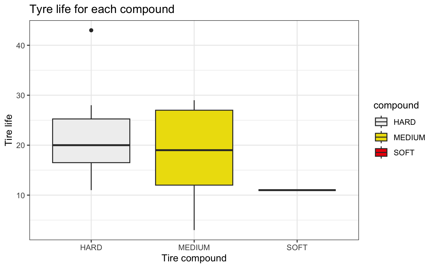 - The plot shows the distribution of tire life (measured in laps) for each tire compound used in the race. On average, hard tires lasted very slightly longer than medium tires. Since hard and medium compounds were the most commonly used in this race, we have limited data on soft tires, roughly a quarter as much. This resulted in a narrower distribution for the soft compound. The tire compound directly affects tire life, with a trade-off between performance (speed and grip) and durability. As a result, softer compounds tend to wear out more quickly than harder ones.
Number of tires for each compound 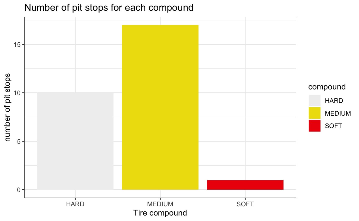 - Since the tire life is shorter for the softer compounds, but has a better performance, the drivers preferred MEDIUM tire to balance the trade-off.
Linear Regression Model
Research questions
- Were drivers more likely to make pit stops when their lap time was longer and their tires were older compared to when their lap time was shorter and their tires were less used?
- Were drivers more likely to make pit stops when their lap times were longer, their tires were older, and considering the type of tires they were using and their progress in the race?
Linear models considering based on the research question
Model 1: \[ \mathbb{E}(pit\_in \mid lap\_time,\ tyre\_life) = \beta_0 + \beta_1(lap\_time) + \beta_2(tyre\_life) \]
Model 2: \[ \begin{aligned} \mathbb{E}(pit\_in \mid lap\_time, \ lap\_number, \ compound, \ tyre\_life) &= \beta_0 + \beta_1(lap\_time) \\ &+ \beta_2(lap\_number) + \beta_3(compound) \\ &+ \beta_4(tyre\_life) \end{aligned} \]
# STEP 1: Model Specification
lm_spec <- linear_reg() %>%
  set_mode("regression") %>%
  set_engine("lm")

# STEP 2: Model estimation
# first linear model
pit_lm1 <- lm_spec %>%
  fit(pit_in ~ lap_time + tyre_life, data = miami2024)
pit_lm1 %>% tidy()
# A tibble: 3 × 5
term estimate std.error statistic p.value
<chr> <dbl> <dbl> <dbl> <dbl>
1 (Intercept) -0.422 0.0543 -7.77 1.74e-14
2 lap_time 0.00429 0.000537 7.98 3.63e-15
3 tyre_life 0.00243 0.000509 4.79 1.94e- 6# second linear model
pit_lm2 <- lm_spec %>%
fit(pit_in ~ lap_time + lap_number + compound + tyre_life, data = miami2024)
pit_lm2 %>% tidy()# A tibble: 6 × 5
term estimate std.error statistic p.value
<chr> <dbl> <dbl> <dbl> <dbl>
1 (Intercept) -0.446 0.0544 -8.21 6.32e-16
2 lap_time 0.00468 0.000534 8.76 7.32e-18
3 lap_number -0.00214 0.000387 -5.54 3.88e- 8
4 compoundMEDIUM 0.0117 0.00936 1.25 2.10e- 1
5 compoundSOFT 0.0312 0.0240 1.30 1.93e- 1
6 tyre_life 0.00519 0.000698 7.44 1.97e-13The regression results show that drivers were slightly more likely to make pit stops when their lap times were longer and their tires were older. In the extended model, lap time and tire age remained strong predictors and suggested that there are fewer stops later in the race with lap number having a slight negative effect. Tire compound had a small and non-significant effect. This indicates that tire compound did not meaningfully influence pit stop decisions when other factors were considered.
Cross Validation
Cross-validation is a statistical method used to evaluate how well a model performs by splitting the data into multiple subsets to train the model on some subsets and validate it on the remaining subsets.
- Goal: Provide a more reliable and unbiased estimate of a model’s performance predicting new data, in order to detect overfitting and improve model generalization
Dividing data into test set and training set
k-fold CV: We can use k-fold cross-validation to estimate the typical error in our model predictions for new data:
- Divide the data into \(k\) folds (or groups) of approximately equal size.
- Repeat the following procedures for each fold \(j = 1,2,...,k\):
- Remove fold \(j\) from the data set.
- Fit a model using the data in the other \(k-1\) folds (training).
- Use this model to predict the responses for the \(n_j\) cases in fold \(j\): \(\hat{y}_1, ..., \hat{y}_{n_j}\).
- Calculate the MAE/MSE for fold \(j\) (testing):
- Combine this information into one measure of model quality
Error metric to use
Mean absolute error (MAE) of an estimator measures the absolute difference between the predicted values and the actual values in the dataset.
- \(\text{MAE}_j = \frac{1}{n_j}\sum_{i=1}^{n_j} |y_i - \hat{y}_i|\)
- \(\text{CV}_{(k)} = \frac{1}{k} \sum_{j=1}^k \text{MAE}_j\)
Mean squared error (MSE) of an estimator measures the average squared difference between the predicted values and the actual values in the dataset.
- \(\text{MSE}_j = \frac{1}{n_j}\sum_{i=1}^{n_j} (y_i - \hat{y}_i)^2\)
- \(\text{CV}_{(k)} = \frac{1}{k} \sum_{j=1}^k \text{MSE}_j\)
MAE vs. MSE
The advantage of using MAE is that it’s more robust to outliers, giving equal weight to all errors. Thus, it’s more suitable when outliers are not a significant concern.
On the other hand, MSE gives more weight to larger errors than smaller ones, making it highly sensitive to outliers. MSE is more suitable when the risk of prediction mistakes is crucial and the goal is to minimize the risk of errors.
Since outliers are less of a concern for us as they don’t lead to any life threatening or other major issues, we prioritize models that are directly interpretable. Our data is less common and less familiar to many people, so we decided to choose a model based on MAE.
pit_lm1 %>% augment(new_data = miami2024) %>%
  mae(truth = pit_in, estimate = .pred)
# A tibble: 1 × 3
.metric .estimator .estimate
<chr> <chr> <dbl>
1 mae standard 0.0505pit_lm2 %>% augment(new_data = miami2024) %>%
mae(truth = pit_in, estimate = .pred)# A tibble: 1 × 3
.metric .estimator .estimate
<chr> <chr> <dbl>
1 mae standard 0.0587k-fold CV implementation for different values of k
k=5
Model 1
# set seed for reproducibility
set.seed(123)

pit_lm1_k5 = lm_spec %>%
  fit_resamples(
    pit_in ~ lap_time + tyre_life,
    resamples = vfold_cv(miami2024, v = 5),
    metrics = metric_set(mae, rmse)
  )
pit_lm1_k5 %>% collect_metrics()
# A tibble: 2 × 6
.metric .estimator mean n std_err .config
<chr> <chr> <dbl> <int> <dbl> <chr>
1 mae standard 0.0507 5 0.00159 Preprocessor1_Model1
2 rmse standard 0.152 5 0.00536 Preprocessor1_Model1# get fold-by-fold results
pit_lm1_k5 %>% unnest(.metrics) %>%
filter(.metric == "mae")# A tibble: 5 × 7
splits id .metric .estimator .estimate .config .notes
<list> <chr> <chr> <chr> <dbl> <chr> <list>
1 <split [884/222]> Fold1 mae standard 0.0477 Preprocessor1_M… <tibble>
2 <split [885/221]> Fold2 mae standard 0.0560 Preprocessor1_M… <tibble>
3 <split [885/221]> Fold3 mae standard 0.0528 Preprocessor1_M… <tibble>
4 <split [885/221]> Fold4 mae standard 0.0486 Preprocessor1_M… <tibble>
5 <split [885/221]> Fold5 mae standard 0.0485 Preprocessor1_M… <tibble>- Based on the random folds above, MAE was best for fold 1 (0.048) and worst for fold 2 (0.056).
Model 2
# set seed for reproducibility
set.seed(123)

pit_lm2_k5 = lm_spec %>%
  fit_resamples(
    pit_in ~ lap_time + lap_number + compound + tyre_life,
    resamples = vfold_cv(miami2024, v = 5),
    metrics = metric_set(mae, rmse)
  )
pit_lm2_k5 %>% collect_metrics()
# A tibble: 2 × 6
.metric .estimator mean n std_err .config
<chr> <chr> <dbl> <int> <dbl> <chr>
1 mae standard 0.0592 5 0.00161 Preprocessor1_Model1
2 rmse standard 0.150 5 0.00490 Preprocessor1_Model1# get fold-by-fold results
pit_lm2_k5 %>% unnest(.metrics) %>%
filter(.metric == "mae")# A tibble: 5 × 7
splits id .metric .estimator .estimate .config .notes
<list> <chr> <chr> <chr> <dbl> <chr> <list>
1 <split [884/222]> Fold1 mae standard 0.0533 Preprocessor1_M… <tibble>
2 <split [885/221]> Fold2 mae standard 0.0621 Preprocessor1_M… <tibble>
3 <split [885/221]> Fold3 mae standard 0.0617 Preprocessor1_M… <tibble>
4 <split [885/221]> Fold4 mae standard 0.0585 Preprocessor1_M… <tibble>
5 <split [885/221]> Fold5 mae standard 0.0606 Preprocessor1_M… <tibble>- Based on the random folds above, MAE was best for fold 1 (0.053) and worst for fold 2 (0.062).
# 5-fold CV MAE and sd
pit_lm1_k5 %>% unnest(.metrics) %>%
  filter(.metric == "mae") %>%
  summarize(mean = mean(.estimate), sd = sd(.estimate))
# A tibble: 1 × 2
mean sd
<dbl> <dbl>
1 0.0507 0.00356pit_lm2_k5 %>% unnest(.metrics) %>%
filter(.metric == "mae") %>%
summarize(mean = mean(.estimate), sd = sd(.estimate))# A tibble: 1 × 2
mean sd
<dbl> <dbl>
1 0.0592 0.00360In-sample and 5-fold CV MAE and standard deviation for both models.
| Model | In-sample MAE | 5-fold CV MAE | In-sample SD | 5-fold CV SD |
|---|---|---|---|---|
model_1 |
0.05045 | 0.05073 | 0.15247 | 0.00356 |
model_2 |
0.05975 | 0.05922 | 0.15035 | 0.00360 |
5-fold cross-validation was used to assess the performance of two models predicting pit stops. Model 1, using only lap time and tire life, achieved a mean MAE of 0.05073 with a low standard deviation (0.00356). Model 2, which adds lap number and tire compound, had a higher mean MAE of 0.05922 with a similar standard deviation (0.00360).
- Although Model 2 includes more predictors, it performed slightly worse than Model 1 in both cross-validation and in-sample metrics. This suggests that the additional variables do not improve prediction. Model 1 is therefore more accurate and efficient for predicting pit stops.
k=10
Model 1
# set seed for reproducibility
set.seed(123)

pit_lm1_cv = lm_spec %>%
  fit_resamples(
    pit_in ~ lap_time + tyre_life,
    resamples = vfold_cv(miami2024, v = 10),
    metrics = metric_set(mae, rmse)
  )
pit_lm1_cv %>% collect_metrics()
# A tibble: 2 × 6
.metric .estimator mean n std_err .config
<chr> <chr> <dbl> <int> <dbl> <chr>
1 mae standard 0.0510 10 0.00294 Preprocessor1_Model1
2 rmse standard 0.150 10 0.0109 Preprocessor1_Model1# get fold-by-fold results
pit_lm1_cv %>% unnest(.metrics) %>%
filter(.metric == "mae")# A tibble: 10 × 7
splits id .metric .estimator .estimate .config .notes
<list> <chr> <chr> <chr> <dbl> <chr> <list>
1 <split [995/111]> Fold01 mae standard 0.0368 Preprocessor1… <tibble>
2 <split [995/111]> Fold02 mae standard 0.0544 Preprocessor1… <tibble>
3 <split [995/111]> Fold03 mae standard 0.0614 Preprocessor1… <tibble>
4 <split [995/111]> Fold04 mae standard 0.0472 Preprocessor1… <tibble>
5 <split [995/111]> Fold05 mae standard 0.0379 Preprocessor1… <tibble>
6 <split [995/111]> Fold06 mae standard 0.0602 Preprocessor1… <tibble>
7 <split [996/110]> Fold07 mae standard 0.0600 Preprocessor1… <tibble>
8 <split [996/110]> Fold08 mae standard 0.0434 Preprocessor1… <tibble>
9 <split [996/110]> Fold09 mae standard 0.0505 Preprocessor1… <tibble>
10 <split [996/110]> Fold10 mae standard 0.0581 Preprocessor1… <tibble>- Based on the random folds above, the MAE was best for fold 1 with an MAE of approximately 0.037 and worst for fold 3 with an MAE of 0.061 approximately.
Model 2
# set seed for reproducibility
set.seed(123)

pit_lm2_cv = lm_spec %>%
  fit_resamples(
    pit_in ~ lap_time + lap_number + compound + tyre_life,
    resamples = vfold_cv(miami2024, v = 10),
    metrics = metric_set(mae, rmse)
  )
pit_lm2_cv %>% collect_metrics()
# A tibble: 2 × 6
.metric .estimator mean n std_err .config
<chr> <chr> <dbl> <int> <dbl> <chr>
1 mae standard 0.0594 10 0.00262 Preprocessor1_Model1
2 rmse standard 0.148 10 0.0104 Preprocessor1_Model1# get fold-by-fold results
pit_lm2_cv %>% unnest(.metrics) %>%
filter(.metric == "mae")# A tibble: 10 × 7
splits id .metric .estimator .estimate .config .notes
<list> <chr> <chr> <chr> <dbl> <chr> <list>
1 <split [995/111]> Fold01 mae standard 0.0436 Preprocessor1… <tibble>
2 <split [995/111]> Fold02 mae standard 0.0616 Preprocessor1… <tibble>
3 <split [995/111]> Fold03 mae standard 0.0698 Preprocessor1… <tibble>
4 <split [995/111]> Fold04 mae standard 0.0566 Preprocessor1… <tibble>
5 <split [995/111]> Fold05 mae standard 0.0518 Preprocessor1… <tibble>
6 <split [995/111]> Fold06 mae standard 0.0658 Preprocessor1… <tibble>
7 <split [996/110]> Fold07 mae standard 0.0655 Preprocessor1… <tibble>
8 <split [996/110]> Fold08 mae standard 0.0521 Preprocessor1… <tibble>
9 <split [996/110]> Fold09 mae standard 0.0601 Preprocessor1… <tibble>
10 <split [996/110]> Fold10 mae standard 0.0671 Preprocessor1… <tibble>- Based on the random folds above, MAE was best for fold 1 (0.044) and worst for fold 3 (0.070).
# 10-fold CV MAE and sd
pit_lm1_cv %>% unnest(.metrics) %>%
  filter(.metric == "mae") %>%
  summarize(mean = mean(.estimate), sd = sd(.estimate))
# A tibble: 1 × 2
mean sd
<dbl> <dbl>
1 0.0510 0.00931pit_lm2_cv %>% unnest(.metrics) %>%
filter(.metric == "mae") %>%
summarize(mean = mean(.estimate), sd = sd(.estimate))# A tibble: 1 × 2
mean sd
<dbl> <dbl>
1 0.0594 0.00829In-sample and 10-fold CV MAE and standard deviation for both models.
| Model | In-sample MAE | 10-fold CV MAE | In-sample SD | 10-fold CV SD |
|---|---|---|---|---|
model_1 |
0.05045 | 0.05100 | 0.15247 | 0.00931 |
model_2 |
0.05975 | 0.05939 | 0.15035 | 0.00829 |
- With 10-fold cross-validation, Model 1 had a mean MAE of 0.0510, while Model 2 had a slightly higher MAE of 0.0594. Both models showed low standard deviations approximately 0.009. As in the 5-fold case, Model 1 remained slightly more accurate and stable than Model 2.
k = 20
Model 1
# set seed for reproducibility
set.seed(123)

pit_lm1_k20 = lm_spec %>%
  fit_resamples(
    pit_in ~ lap_time + tyre_life,
    resamples = vfold_cv(miami2024, v = 20),
    metrics = metric_set(mae, rmse)
  )
pit_lm1_k20 %>% collect_metrics()
# A tibble: 2 × 6
.metric .estimator mean n std_err .config
<chr> <chr> <dbl> <int> <dbl> <chr>
1 mae standard 0.0509 20 0.00399 Preprocessor1_Model1
2 rmse standard 0.140 20 0.0142 Preprocessor1_Model1# get fold-by-fold results
pit_lm1_k20 %>% unnest(.metrics) %>%
filter(.metric == "mae")# A tibble: 20 × 7
splits id .metric .estimator .estimate .config .notes
<list> <chr> <chr> <chr> <dbl> <chr> <list>
1 <split [1050/56]> Fold01 mae standard 0.0451 Preprocessor1… <tibble>
2 <split [1050/56]> Fold02 mae standard 0.0519 Preprocessor1… <tibble>
3 <split [1050/56]> Fold03 mae standard 0.0509 Preprocessor1… <tibble>
4 <split [1050/56]> Fold04 mae standard 0.0658 Preprocessor1… <tibble>
5 <split [1050/56]> Fold05 mae standard 0.0439 Preprocessor1… <tibble>
6 <split [1050/56]> Fold06 mae standard 0.0412 Preprocessor1… <tibble>
7 <split [1051/55]> Fold07 mae standard 0.0602 Preprocessor1… <tibble>
8 <split [1051/55]> Fold08 mae standard 0.0429 Preprocessor1… <tibble>
9 <split [1051/55]> Fold09 mae standard 0.0402 Preprocessor1… <tibble>
10 <split [1051/55]> Fold10 mae standard 0.0263 Preprocessor1… <tibble>
11 <split [1051/55]> Fold11 mae standard 0.0266 Preprocessor1… <tibble>
12 <split [1051/55]> Fold12 mae standard 0.0585 Preprocessor1… <tibble>
13 <split [1051/55]> Fold13 mae standard 0.0704 Preprocessor1… <tibble>
14 <split [1051/55]> Fold14 mae standard 0.0274 Preprocessor1… <tibble>
15 <split [1051/55]> Fold15 mae standard 0.0302 Preprocessor1… <tibble>
16 <split [1051/55]> Fold16 mae standard 0.0825 Preprocessor1… <tibble>
17 <split [1051/55]> Fold17 mae standard 0.0591 Preprocessor1… <tibble>
18 <split [1051/55]> Fold18 mae standard 0.0429 Preprocessor1… <tibble>
19 <split [1051/55]> Fold19 mae standard 0.0611 Preprocessor1… <tibble>
20 <split [1051/55]> Fold20 mae standard 0.0901 Preprocessor1… <tibble>- Based on the random folds above, MAE was best for fold 10 (0.026) and worst for fold 20 (0.090).
Model 2
# set seed for reproducibility
set.seed(123)

pit_lm2_k20 = lm_spec %>%
  fit_resamples(
    pit_in ~ lap_time + lap_number + compound + tyre_life,
    resamples = vfold_cv(miami2024, v = 20),
    metrics = metric_set(mae, rmse)
  )
pit_lm2_k20 %>% collect_metrics()
# A tibble: 2 × 6
.metric .estimator mean n std_err .config
<chr> <chr> <dbl> <int> <dbl> <chr>
1 mae standard 0.0593 20 0.00398 Preprocessor1_Model1
2 rmse standard 0.139 20 0.0134 Preprocessor1_Model1# get fold-by-fold results
pit_lm2_k20 %>% unnest(.metrics) %>%
filter(.metric == "mae")# A tibble: 20 × 7
splits id .metric .estimator .estimate .config .notes
<list> <chr> <chr> <chr> <dbl> <chr> <list>
1 <split [1050/56]> Fold01 mae standard 0.0508 Preprocessor1… <tibble>
2 <split [1050/56]> Fold02 mae standard 0.0623 Preprocessor1… <tibble>
3 <split [1050/56]> Fold03 mae standard 0.0564 Preprocessor1… <tibble>
4 <split [1050/56]> Fold04 mae standard 0.0755 Preprocessor1… <tibble>
5 <split [1050/56]> Fold05 mae standard 0.0596 Preprocessor1… <tibble>
6 <split [1050/56]> Fold06 mae standard 0.0535 Preprocessor1… <tibble>
7 <split [1051/55]> Fold07 mae standard 0.0652 Preprocessor1… <tibble>
8 <split [1051/55]> Fold08 mae standard 0.0492 Preprocessor1… <tibble>
9 <split [1051/55]> Fold09 mae standard 0.0474 Preprocessor1… <tibble>
10 <split [1051/55]> Fold10 mae standard 0.0324 Preprocessor1… <tibble>
11 <split [1051/55]> Fold11 mae standard 0.0347 Preprocessor1… <tibble>
12 <split [1051/55]> Fold12 mae standard 0.0630 Preprocessor1… <tibble>
13 <split [1051/55]> Fold13 mae standard 0.0818 Preprocessor1… <tibble>
14 <split [1051/55]> Fold14 mae standard 0.0362 Preprocessor1… <tibble>
15 <split [1051/55]> Fold15 mae standard 0.0405 Preprocessor1… <tibble>
16 <split [1051/55]> Fold16 mae standard 0.0838 Preprocessor1… <tibble>
17 <split [1051/55]> Fold17 mae standard 0.0652 Preprocessor1… <tibble>
18 <split [1051/55]> Fold18 mae standard 0.0537 Preprocessor1… <tibble>
19 <split [1051/55]> Fold19 mae standard 0.0724 Preprocessor1… <tibble>
20 <split [1051/55]> Fold20 mae standard 0.102 Preprocessor1… <tibble>- Based on the random folds above, MAE was best for fold 10 (0.032) and worst for fold 20 (0.101).
# 20-fold CV MAE and sd
pit_lm1_k20 %>% unnest(.metrics) %>%
  filter(.metric == "mae") %>%
  summarize(mean = mean(.estimate), sd = sd(.estimate))
# A tibble: 1 × 2
mean sd
<dbl> <dbl>
1 0.0509 0.0178pit_lm2_k20 %>% unnest(.metrics) %>%
filter(.metric == "mae") %>%
summarize(mean = mean(.estimate), sd = sd(.estimate))# A tibble: 1 × 2
mean sd
<dbl> <dbl>
1 0.0593 0.0178In-sample and 20-fold CV MAE and standard deviation for both models.
| Model | In-sample MAE | 20-fold CV MAE | In-sample SD | 20-fold CV SD |
|---|---|---|---|---|
model_1 |
0.05045 | 0.05086 | 0.15247 | 0.01785 |
model_2 |
0.05975 | 0.05925 | 0.15035 | 0.01781 |
- In the 20-fold CV setup, Model 1 performed better than Model 2 with a lower mean MAE, 0.05086 and 0.05925, respectively. Even with increased fold, the simpler model generalized better across the dataset.
Compare different values of k
| Model | In-sample MAE | 5-fold CV MAE | 10-fold CV MAE | 20-fold CV MAE |
|---|---|---|---|---|
model_1 |
0.05045 | 0.05073 | 0.05100 | 0.05086 |
model_2 |
0.05975 | 0.05922 | 0.05939 | 0.05925 |
Final model based on the smallest CV error
Across all cross-validation settings (5, 10, and 20-fold), Model 1 consistently showed lower MAE than Model 2. The differences were small but consistent and this suggests that Model 1 is a better model than Model 2 in predicting pit-stops.
Therefore, our final model based on the smallest CV error is:
\[ \mathbb{E}(pit\_in \mid lap\_time,\ tyre\_life) = \beta_0 + \beta_1(lap\_time) + \beta_2(tyre\_life) \]
Logistic Regression Model
Variables of interest
Predictors
lap_time: recorded time to complete a lap (seconds)lap_number: lap number from which the telemetry data was recorded (number of laps)tyre_life: number of laps completed on a set of tires (number of laps)compound: type of tire used (SOFT, MEDIUM, HARD)
Response variable
pit_in: whether a driver made a pit stop during a lap (binary: 0 = no pit stop, 1 = pit stop occurred)\[\begin{align*} Y_i &= \begin{cases} 1 & \text{ if a driver pitted on a lap } \\ 0 & \text{ otherwise (i.e., the driver did not pit on lap)} \end{cases} \end{align*}\]
Our logistic regression model
We are interested in determining the probability of making a pit stop during the 2024 Miami Grand Prix, considering factors such as lap time, track progress, tire age, and the type of tire used.
\[ \begin{aligned} \log(odds(pit\_in \mid lap\_time, \ lap\_number, \ tyre\_life, \ compound)) &= \beta_0 + \beta_1 (lap\_time) \\ &+ \beta_2(lap\_number) + \beta_3 (tyre\_life) \\ &+ \beta_4 \ I(compound = MEDIUM) \\ &+ \beta_5 \ I(compound = SOFT) \end{aligned} \]
# factor `pit_in` for logistic regression analysis
miami2024_glm <- miami2024 %>%
  mutate(pit_in_fac = as.factor(pit_in))
# logistic regression model
logistic_fit <- train(
form = pit_in_fac ~ lap_time + lap_number + tyre_life + compound,
data = miami2024_glm,
family = "binomial", # this is an argument to glm; response is 0 or 1, binomial
method = "glm", # method for fit; "generalized linear model"
trControl = trainControl(method = "none")
)
summary(logistic_fit$finalModel)
Call:
NULL

Coefficients:
                Estimate Std. Error z value Pr(>|z|)
(Intercept)    -18.48162    2.27137  -8.137 4.06e-16 ***
lap_time         0.13739    0.02007   6.846 7.58e-12 ***
lap_number      -0.16001    0.03630  -4.408 1.04e-05 ***
tyre_life        0.27508    0.04580   6.006 1.91e-09 ***
compoundMEDIUM   0.49495    0.49718   0.996    0.319
compoundSOFT     1.86135    1.17923   1.578    0.114
---
Signif. codes:  0 '***' 0.001 '**' 0.01 '*' 0.05 '.' 0.1 ' ' 1

(Dispersion parameter for binomial family taken to be 1)

    Null deviance: 261.16  on 1105  degrees of freedom
Residual deviance: 176.46  on 1100  degrees of freedom
AIC: 188.46

Number of Fisher Scoring iterations: 8
Interpretation of exponentiated \(\hat{\beta}\) coefficients
exp(logistic_fit$finalModel$coefficients) (Intercept) lap_time lap_number tyre_life compoundMEDIUM
9.408757e-09 1.147280e+00 8.521343e-01 1.316630e+00 1.640419e+00
compoundSOFT
6.432386e+00 \(\exp(\beta_0)\): The odds of a driver making a pit stop during a lap, when lap time is 0 seconds, lap number is 0, 0 laps have been completed on the current set of tires, and the HARD compound is, is approximately \(9.4088 \times 10^{-9}\).
\(\exp(\beta_1)\): For every of 1 second increase in lap time, the odds of a driver pitting increase by a factor of 1.1473.
\(\exp(\beta_2)\): For every additional lap (i.e., increase of 1 in the lap number), we expect the odds of a driver pitting to increase by a factor of 0.8521.
\(\exp(\beta_3)\): For each additional lap completed on the current set of tires, the odds of a driver pitting increase by a factor of 1.3166.
\(\exp(\beta_4)\): When using MEDIUM compound tires instead of HARD, the odds of a driver pitting increase by a factor of 1.6404, holding all other variables constant.
\(\exp(\beta_5)\): When using SOFT compound tires instead of HARD, we expect the odds of a driver pitting to increase by a factor of 6.4324, holding all other variables constant.
Mathematically derive \(\exp(\beta_1)\)
\[ \begin{aligned} &\log(odds(pit\_in \mid lap\_time = a)) = -18.4816 + 0.1374a \\ \\ &\log(odds(pit\_in \mid lap\_time = a+1)) = -18.4816 + 0.1374(a+1) \end{aligned} \]
\[ \begin{aligned} & \log\left( \frac{odds(pit\_in \mid lap\_time = a+1)}{odds(pit\_in \mid lap\_time = a)} \right)\\ &= \log(odds(pit\_in \mid lap\_time = a+1)) - \log(odds(pit\_in \mid lap\_time = a)) \\ &= (-18.4816 + 0.1374(a+1)) - (-18.4816 + 0.1374) \\ &= 0.1374 \\ &= \hat{\beta_1} \end{aligned} \]
Therefore, \(\exp(\beta_1) = e^{0.1374} = 1.1473\)
Predicting High Probability of a Pit Stop
To predict a probability of a driver making a pit stop that is very close to 1, we need to input extreme values for the predictors. Based on the five-number summary of our data, we use the following scenario: a lap time of 148.74 seconds, lap number 57, SOFT compound, and a tire age of 45 laps.
# miami2024_glm %>%
#   ggplot(aes(x=lap_time)) +
#     geom_density(fill="#69b3a2", color="#e9ecef", alpha=0.8)

summary(miami2024_glm)
lap_time lap_number compound tyre_life
Min. : 90.63 Min. : 1.00 HARD :500 Min. : 1.00
1st Qu.: 92.38 1st Qu.:14.00 MEDIUM:562 1st Qu.: 7.00
Median : 93.28 Median :28.00 SOFT : 44 Median :13.50
Mean : 96.00 Mean :28.62 Mean :14.78
3rd Qu.: 94.29 3rd Qu.:43.00 3rd Qu.:22.00
Max. :148.74 Max. :57.00 Max. :45.00
pit_in pit_in_fac
Min. :0.00000 0:1078
1st Qu.:0.00000 1: 28
Median :0.00000
Mean :0.02532
3rd Qu.:0.00000
Max. :1.00000 log_prid_fst <- predict(logistic_fit$finalModel,
newdata = data.frame(lap_time = 148.74,
lap_number = 57,
tyre_life = 45,
compoundMEDIUM = 0,
compoundSOFT = 1),
type = "response")
odds_pitting_fst = exp(log_prid_fst)
(prob_pitting_fst = odds_pitting_fst/(1+odds_pitting_fst)) 1
0.7308921 Using our logistic regression model, we estimate the probability of a pit stop under these conditions to be approximately 0.731. This indicates a high likelihood of a pit stop given these extreme race conditions.
Predicting Pit Stops with our Logistic Regression Model
Estimate the probability of a driver making a pit stop on a lap with the following conditions: 96.00 seconds lap time, 28th lap, 14.78 laps completed on a set of HARD tires.
log_prid_hard <- predict(logistic_fit$finalModel,
        newdata = data.frame(lap_time = 96,
                             lap_number = 28,
                             tyre_life = 14.78,
                             compoundMEDIUM = 0,
                             compoundSOFT = 0),
        type = "response")

odds_pitting_hard = exp(log_prid_hard)
(prob_pitting_hard = odds_pitting_hard/(1+odds_pitting_hard))
1 0.5008283
There is approximately a 50.08% probability that a driver will make a pit stop on this lap when using HARD tires, holding all other variables constant.
Estimate the probability of a driver making a pit stop on a lap under the same conditions as above but using a set of MEDIUM tires.
log_prid_med <- predict(logistic_fit$finalModel,
        newdata = data.frame(lap_time = 96,
                             lap_number = 28,
                             tyre_life = 14.78,
                             compoundMEDIUM = 1,
                             compoundSOFT = 0),
        type = "response")

odds_pitting_med = exp(log_prid_med)
(prob_pitting_med = odds_pitting_med/(1+odds_pitting_med))
1 0.5013559
With MEDIUM tires, the probability of making a pit stop increases to 50.14%.
Estimate the probability of a driver making a pit stop on a lap under the same conditions as above but using a set of SOFT tires.
log_prid_soft <- predict(logistic_fit$finalModel,
        newdata = data.frame(lap_time = 96,
                             lap_number = 28,
                             tyre_life = 14.78,
                             compoundMEDIUM = 0,
                             compoundSOFT = 1),
        type = "response")

odds_pitting_soft = exp(log_prid_soft)
(prob_pitting_soft = odds_pitting_soft/(1+odds_pitting_soft))
1 0.5052337
With SOFT tires, the probability increases slightly to 50.52%.
While all the other variables stay the same, we predict that the probability a driver to made a pit stop is higher if the driver is on a set of SOFT tires compared to other compounds.
Pros/Cons of logistic regression vs. regular linear regression
Logistic Regression
| Pros | Since logistic regression is based on a Bernoulli/binomial likelihood, it is a natural model for binary outcomes. Coefficients are interpretable in terms of odds ratios (with log-odds as the linear predictor). |
| Cons | The relationship between predictors and the probability is not linear. |
Linear Regression
| Pros | Straightforward linear regression Easy to interpret the coefficients |
| Cons | Cannot gaurantee that the predicted probabilities to be between 0 and 1. |
Conclusion
The linear and logistic regression models provide a practical method for predicting pit-stop laps based on multiple factors, while k-fold cross-validation offers an approach for selecting the most optimized models. However, the prediction results from the logistic model were somewhat limited, with predictions averaging around 50% even with extreme parameters, making it challenging to accurately predict pit-stop laps. This limitation is understandable because predicting pit-stop timing in real races is one of the most crucial and difficult decisions in race strategy.
For future studies, we could consider additional factors that influence car speeds or tire management, as well as apply methods that are capable of handling more complex models to observed more detailed and comprehensive analyses.